Machine Learning Starting Blocks

I've not written about my experience in Machine Learning at all. As a Student I studied the algorithms and proofs to back up many modeling techniques. As far as my professional role as a Senior Engineer goes, I've at least dabbled in most mainstream tools out there. And as a Senior Data Engineer, I've focused recently on the applications of tools in the data space, including modelling, munging and machine learning. This post is more of a refresher - something I can refer back to in order to quickly get back running on a project where at least a simplistic overview is required.

So what will I detail in the end? I'd like to show that ML in this post (and in most rudimentary models) is essentially curve fitting for lack of better words. The machine is learning how to predict a value y, based on a set of input variables x. This post isn't meant to break the bounds of ML, here x is just a tuple of floats, a set of numeric values that describe the underlying data. We don't go into handling categories or more structured, contextual data such as time-series or natural language.

By the end, you'll have seen, at least from a regression point of view, a way of understanding goals and how models may be more accustomed to solving certain problems. If this interests me enough I might do a second part on how the underlying models work, or we could just jump into neural models and skip the old school ML. Side note: I'd like to do a history of ML at some point too.

Getting Started

The first bits of python is always meta executions, setting up libs and the like - ill comment on what's going on at each point.

The first cell contains commented out operations to install the notebook deps - I operate locally and use poetry for deps, the poetry.toml is in an appendix.

It's worth noting this was written in a jupyter notebook

1
2
3
4
5
6
# !pip install pandas=="^1.4.0"
# !pip install plotly=="^5.5.0"
# !pip install scikit-learn=="^1.0.2"
# !pip install kaggle=="^1.5.12"
# !pip install jupyter=="^1.0.0"
# !pip install seaborn=="^0.11.2"

1
2
3
4
5
6
7
8
9
10
11
12
13
14
15
16
17
18
# various imports, google for info
import time
import timeit

import pandas as pd
import numpy as np
import seaborn as sns
import matplotlib.pyplot as plt

# default plot to sns and style to be nicer to the eyes in dark mode
sns.set_theme(
    context='notebook', style='darkgrid', color_codes=True,
    font_scale=1.5, rc={'figure.figsize': (20, 10)}
)

# reproducibility
SEED = 1234
np.random.seed(SEED)

1
2
3
# Magic lines like this mean we can set notebook properties, see below for more
# https://ipython.readthedocs.io/en/stable/interactive/magics.html
# %config InlineBackend.figure_format = 'svg'

Data download

data should be extracted to the /data dir, it's from kaggles housesalesprediction dataset, a great resource for learning ML. I hope you stumbled across that website before this post. To set up run the below, this will pull down a zip of the files we want. You'll need to unzip and place in the format below.

poetry run kaggle datasets download -d harlfoxem/housesalesprediction

1
2
3
4
5
/data
/...
/kc_house_data.csv
/- ...
/house_prices.ipynb

Looking at the data

This next section looks at the data in the resulting CSV. As far as data goes its lovely, with no horrible decisions we need to make about munging. in the real world this next step is much more important and can change the results from a mediocre model to an amazing one. Data is the fuel of the ML flame, wet kindling will give shitty results.

There are a few things I like to look for in data munging tabular records:

1. **Overall size ** - ideally this should be known before loading the data into memory and potentially an iterative approach to be designed using chunking.
2. **Num columns ** - is our dimensionality huge? would removing a large number impact us? are there any highly correlated cols? what about synthetic variables?
3. **Column types ** - are we going to have trouble with certain fields (dates, non UTF-8 chars, serialized/nested fields, badly typed fields)
4. **Column names ** - is there a description of what's in that column? something I can sanity check with external data maybe? £50 house prices would raise alarms.
5. Null/missing data - how will we deal with these records? are the null records a large chunk of the data?

Ideally, this non-exhaustive list of checks should be completed upstream in our stack by tools such as dbt. As a Data scientist, I want to have a reproducible way of cleaning my data.

1
2
df = pd.read_csv('data/kc_house_data.csv')
df.info()

1
2
3
4
5
6
7
8
9
10
11
12
13
14
15
16
17
18
19
20
21
22
23
24
25
26
27
28
<class 'pandas.core.frame.DataFrame'>
RangeIndex: 21613 entries, 0 to 21612
Data columns (total 21 columns):
 #   Column         Non-Null Count  Dtype
---  ------         --------------  -----
 0   id             21613 non-null  int64
 1   date           21613 non-null  object
 2   price          21613 non-null  float64
 3   bedrooms       21613 non-null  int64
 4   bathrooms      21613 non-null  float64
 5   sqft_living    21613 non-null  int64
 6   sqft_lot       21613 non-null  int64
 7   floors         21613 non-null  float64
 8   waterfront     21613 non-null  int64
 9   view           21613 non-null  int64
 10  condition      21613 non-null  int64
 11  grade          21613 non-null  int64
 12  sqft_above     21613 non-null  int64
 13  sqft_basement  21613 non-null  int64
 14  yr_built       21613 non-null  int64
 15  yr_renovated   21613 non-null  int64
 16  zipcode        21613 non-null  int64
 17  lat            21613 non-null  float64
 18  long           21613 non-null  float64
 19  sqft_living15  21613 non-null  int64
 20  sqft_lot15     21613 non-null  int64
dtypes: float64(5), int64(15), object(1)
memory usage: 3.5+ MB

1
df.sort_values('id').head()

1
2
3
4
5
6
7
|      |   id    | date                | price  | bedrooms | bathrooms | sqft_living | sqft_lot | floors | waterfront | view | condition | grade | sqft_above | sqft_basement | yr_built | yr_renovated | zipcode |   lat   |   long   | sqft_living15 | sqft_lot15 |
|:----:|:-------:|:--------------------|:------:|:--------:|:---------:|:-----------:|:--------:|:------:|:----------:|:----:|:---------:|:-----:|:----------:|:-------------:|:--------:|:------------:|:-------:|:-------:|:--------:|:-------------:|:----------:|
| 2497 | 1000102 | 2015-04-22 00:00:00 | 300000 |    6     |     3     |    2400     |   9373   |   2    |     0      |  0   |     3     |   7   |    2400    |       0       |   1991   |      0       |  98002  | 47.3262 | -122.214 |     2060      |    7316    |
| 2496 | 1000102 | 2014-09-16 00:00:00 | 280000 |    6     |     3     |    2400     |   9373   |   2    |     0      |  0   |     3     |   7   |    2400    |       0       |   1991   |      0       |  98002  | 47.3262 | -122.214 |     2060      |    7316    |
| 6735 | 1200019 | 2014-05-08 00:00:00 | 647500 |    4     |   1.75    |    2060     |  26036   |   1    |     0      |  0   |     4     |   8   |    1160    |      900      |   1947   |      0       |  98166  | 47.4444 | -122.351 |     2590      |   21891    |
| 8411 | 1200021 | 2014-08-11 00:00:00 | 400000 |    3     |     1     |    1460     |  43000   |   1    |     0      |  0   |     3     |   7   |    1460    |       0       |   1952   |      0       |  98166  | 47.4434 | -122.347 |     2250      |   20023    |
| 8809 | 2800031 | 2015-04-01 00:00:00 | 235000 |    3     |     1     |    1430     |   7599   |  1.5   |     0      |  0   |     4     |   6   |    1010    |      420      |   1930   |      0       |  98168  | 47.4783 | -122.265 |     1290      |   10320    |

Looks like our data is clean - we have 20 columns where only some don't make sense. All the values are numeric apart from date, which looks like a ISO 8061 string representation, which makes it easy for us to parse. Some of these can be classified as categories under the hood, so we could try One Hot Encoding them later after a baseline is expected. There are lots of years in here that could also be better off converted to relative values, a zip code that's represented as a number and lat-long values which could be geo-aizied too. Location data as a concept is layered and in this case we may be better off ignoring some of them, well come to selecting data later. For now we are not going to touch the data other than the date to get it in the right format.

One thing to note is that this set of data contains multiple sales of the same house, for example house 1000102 which sold for $280,000 in 2014 then in 2015 for $300,000. This is something that should be incorporated into the model somehow, maybe in a synthetic field further down the line wrt the price - maybe some inflation adjusted value.

1
df['date'] = pd.to_datetime(df['date'])

Data Distribution

As I mentioned this is a very easy data source to begin with, and it's a nice sample to understand too. Everyone understands (apart from the market obviously, as a first time buyer) how a house should be valued at a high level; big => ££, beds => $$ location => €€.

1
df.describe()

1
2
3
4
5
6
7
8
9
10
|       |     id      |  price  | bedrooms | bathrooms | sqft_living |  sqft_lot   |  floors  | waterfront |   view   | condition |  grade  | sqft_above | sqft_basement | yr_built | yr_renovated | zipcode |   lat    |   long   | sqft_living15 | sqft_lot15 |
|:------|:-----------:|:-------:|:--------:|:---------:|:-----------:|:-----------:|:--------:|:----------:|:--------:|:---------:|:-------:|:----------:|:-------------:|:--------:|:------------:|:-------:|:--------:|:--------:|:-------------:|:----------:|
| count |    21613    |  21613  |  21613   |   21613   |    21613    |    21613    |  21613   |   21613    |  21613   |   21613   |  21613  |   21613    |     21613     |  21613   |    21613     |  21613  |  21613   |  21613   |     21613     |   21613    |
| mean  | 4.5803e+09  | 540088  | 3.37084  |  2.11476  |   2079.9    |    15107    | 1.49431  | 0.00754176 | 0.234303 |  3.40943  | 7.65687 |  1788.39   |    291.509    | 1971.01  |   84.4023    | 98077.9 | 47.5601  | -122.214 |    1986.55    |  12768.5   |
| std   | 2.87657e+09 | 367127  | 0.930062 | 0.770163  |   918.441   |   41420.5   | 0.539989 | 0.0865172  | 0.766318 | 0.650743  | 1.17546 |  828.091   |    442.575    | 29.3734  |   401.679    | 53.505  | 0.138564 | 0.140828 |    685.391    |  27304.2   |
| min   | 1.0001e+06  |  75000  |    0     |     0     |     290     |     520     |    1     |     0      |    0     |     1     |    1    |    290     |       0       |   1900   |      0       |  98001  | 47.1559  | -122.519 |      399      |    651     |
| 25%   | 2.12305e+09 | 321950  |    3     |   1.75    |    1427     |    5040     |    1     |     0      |    0     |     3     |    7    |    1190    |       0       |   1951   |      0       |  98033  |  47.471  | -122.328 |     1490      |    5100    |
| 50%   | 3.90493e+09 | 450000  |    3     |   2.25    |    1910     |    7618     |   1.5    |     0      |    0     |     3     |    7    |    1560    |       0       |   1975   |      0       |  98065  | 47.5718  | -122.23  |     1840      |    7620    |
| 75%   | 7.3089e+09  | 645000  |    4     |    2.5    |    2550     |    10688    |    2     |     0      |    0     |     4     |    8    |    2210    |      560      |   1997   |      0       |  98118  |  47.678  | -122.125 |     2360      |   10083    |
| max   |   9.9e+09   | 7.7e+06 |    33    |     8     |    13540    | 1.65136e+06 |   3.5    |     1      |    4     |     5     |   13    |    9410    |     4820      |   2015   |     2015     |  98199  | 47.7776  | -121.315 |     6210      |   871200   |

1
2
heatmap = sns.heatmap(df.corr(), annot=True, fmt=".2f")
heatmap

1
2
pairplot = sns.pairplot(df)
pairplot

1
2
hist = df.hist()
plt.tight_layout()

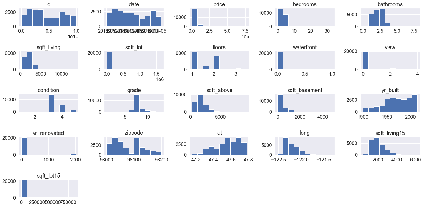
Eyeballing the columns look like everything looks fine, there are some distributions are clearly one sides such as the renovation year & waterfront, view and sqft_lot. Its worth looking into these a little more, see if they'll be useful. There are some clear correlations on some vars, ignoring the price column as that's our y column, looks like there are sqft to sqft columns and bathrooms to sqft. Ultimately these make sense, so we will continue without removing/altering any of these.

There are some that I'd like to look into in more depth, namely

• sqft_lot - why is this all bunched up at the 0 end?
• waterfront - what do these numbers mean?
• view - what do these numbers mean?
• yr_renovated - how does this impact us if we move to relative dates?

1
2
3
4
5
6
7
8
9
10
11
12
13
14
keys = [
    'sqft_lot',
    'waterfront',
    'view',
    'yr_renovated'
]
for key in keys:
    unique_vals = df[key].unique()
    print(f"{key} has {len(unique_vals)} unique values, first 5: {unique_vals[:5]}")

# sqft_lot has 9782 unique values, first 5: [ 5650  7242 10000  5000  8080]
# waterfront has 2 unique values, first 5: [0 1]
# view has 5 unique values, first 5: [0 3 4 2 1]
# yr_renovated has 70 unique values, first 5: [   0 1991 2002 2010 1999]

1
2
3
4
5
6
7
8
9
10
11
12
13
14
15
16
17
18
19
20
21
22
23
24
25
26
27
28
29
30
31
32
33
print("skew:", df.skew()['sqft_lot'])
# skew: 13.060018959031755

print(df['sqft_lot'].describe())
# count    2.161300e+04
# mean     1.510697e+04
# std      4.142051e+04
# min      5.200000e+02
# 25%      5.040000e+03
# 50%      7.618000e+03
# 75%      1.068800e+04
# max      1.651359e+06
# Name: sqft_lot, dtype: float64

print("top 15 values by count")
# top 15 values by count
print(df['sqft_lot'].value_counts()[:15])
# 5000    358
# 6000    290
# 4000    251
# 7200    220
# 4800    120
# 7500    119
# 4500    114
# 8400    111
# 9600    109
# 3600    103
# 9000     93
# 3000     84
# 5100     78
# 7000     76
# 8000     76
# Name: sqft_lot, dtype: int64

Ok looks like we do have some categories in waterfront and view - though as they're encoded already I'll just leave them. sqft_lot looks lie its incredibly sqewed with the majority of the values below 10,000 and a max value of over 150x that. Im not too concerned as this probably has relevent data in, just with an intresting distribution.

Next is to train a basic model as a baseline. As per the basic tutorial ill just use a decision tree as it's relatively easy to understand.

Running Experiments

We will run the following experiments:

1. The first will use the default model with the original, relevant data.
2. We will then tune the hyper-parameters for the model.
3. Then we can apply some data transforms based on the decisions above and try steps 1) and 2) again.

It's worth noting, for now, we will only be doing regression analysis rather than classification. We could bucket the properties into categories then run a classifier on them, however that can be another post.

The prerequisites for doing this is to define our test/train splits and our model grading strategy, to ensure an accurate model. To do this I will define a function that can be reused.

1
2
3
4
5
6
7
8
9
10
11
12
13
14
15
16
17
18
19
from sklearn.model_selection import train_test_split


def get_data(_df=df, seed=SEED):
    _dim_predict = ['price']
    _dim_features = list(
        # Typically, ill remove columns rather than add them together when the dimensionality is small
        set(df.columns) - set(_dim_predict) - {
            # this is just a unique id, as noted this means we may have multiple sales of the same house in the data
            'id',
        }
    )

    _x = _df[_dim_features]
    _y = _df[_dim_predict]

    # easy split of the data in a reproducible.
    _x_train, _x_test, _y_train, _y_test = train_test_split(_x, _y, random_state=seed)
    return _x_train, _x_test, _y_train, _y_test

When it comes to getting the predictions we want to ensure we measure a relevant accuracy. There are lots of ways of doing this for regression, as discussed in this post and in the sklearn docs. Essentially the question is the same:

how far away from the correct answer am I?

This means answering things like penalizing "distance" from the true result, by squaring or just getting the absolute value of the distance and how to aggregate all our guesses, such as taking averages or min/max of our deltas. In my case, I'll try 3:

• Mean Absolute Error ($MAE$)
• Max Error ($ME$)
• Root Mean Squared Error ($RMSE$)

It's worth noting this is just a way of comparing 2 arrays of the same length. We could go into lots of detail around skewness and how that impacts predictions on very expensive/cheap houses or the bulk of our data. Grading a regression model is really important for analysing what, exactly, you want to be predicted from an ML model.

In real terms this means "given all my guesses, how much did I miss the mark by if I were to guess the cost of the house?". For example, if I had a $MAE$ of 50,000 I would interpret that as "given any price guess, I would be about 50,000 dollars off the mark"; a $RMSE$ is the same but would be calculated directly as errors are squared before averaging rather than just the abs value. A $ME$ would be just mean my guesses were within 50,000 dollars at all points, so that's the best upper bound I could expect (well kinda, this isn't the best analysis model). I'd expect the following:

$$ MAE < ME < RMSE $$

I will also return the mean value of the true prices to compare how the model performance actually stacks up

1
2
3
4
5
6
7
8
9
10
11
12
13
14
15
16
17
from sklearn.metrics import mean_absolute_error, mean_squared_error, max_error


def get_errors(y_true, y_predict):
    _mae = mean_absolute_error(y_true, y_predict)
    _me = max_error(y_true, y_predict)
    _rmse = mean_squared_error(y_true, y_predict, squared=False)
    mean = np.mean(y_true.values)
    return {
        'MAE': _mae,
        'MAE_ratio': _mae / mean,
        'ME': _me,
        'ME_ratio': _me / mean,
        'RMSE': _rmse,
        'RMSE_ratio': _rmse / mean,
        'y_true_mean': mean  # sanity check
    }

Modelling

Step one, is the basic Linear Regression. Probably going to not work super well as the data is likely non-linear

1
2
3
4
5
6
7
8
9
10
11
12
13
14
15
16
17
from sklearn.linear_model import LinearRegression

# we expect numerical values for all dimensions
df_lr = df.copy()
df_lr['date'] = pd.to_numeric(df_lr['date'])  # this is converted to a unix timestamp

# Fetch our data to start
x_train, x_test, y_train, y_test = get_data(df_lr)

# training the model
linear_regressor = LinearRegression()
linear_regressor.fit(x_train, y_train)

# get a prediction result
y_pred = linear_regressor.predict(x_test)
linear_result = get_errors(y_test, y_pred)
linear_result

1
2
3
4
5
6
7
{'MAE': 162853.0350747235,
 'MAE_ratio': 0.302607784870751,
 'ME': 4157759.6482200027,
 'ME_ratio': 7.725802817218291,
 'RMSE': 238675.029580604,
 'RMSE_ratio': 0.44349754962938126,
 'y_true_mean': 538165.3850851221}

From here let's try a bunch of other regression modelling techniques to see what the best default is.

1
2
3
4
5
6
7
8
9
10
11
12
13
14
15
16
17
18
19
20
21
22
23
24
25
import time


# this is how we test a single model, and produce a set of metrics to be measured.
def do_basic_model_fitting(regressor):
    start = time.perf_counter_ns()

    _dt = df.copy()
    _dt['date'] = pd.to_numeric(_dt['date'])
    _x_train, _x_test, _y_train, _y_test = get_data(_dt)

    regressor.fit(_x_train, np.ravel(_y_train))

    _y_pred = regressor.predict(_x_test)
    return {'model': str(regressor).strip(), 'time_taken': (time.perf_counter_ns() - start),
            **get_errors(_y_test, _y_pred)}


# function for testing & aggregating multiple model tests
def model_testing(_models):
    test_results = []
    for model in models_1:
        res = do_basic_model_fitting(model)
        test_results.append(res)
    return pd.DataFrame(data=test_results)

1
2
3
4
5
6
7
8
9
10
11
12
13
14
15
16
17
18
19
from sklearn.gaussian_process import GaussianProcessRegressor
from sklearn.tree import DecisionTreeRegressor
from sklearn.ensemble import RandomForestRegressor, GradientBoostingRegressor
from sklearn.neighbors import KNeighborsRegressor
from sklearn.svm import SVR
from sklearn.neural_network import MLPRegressor

# random_state is set with np.random.seed() in one of the top cells.
models_1 = [
    GaussianProcessRegressor(random_state=SEED),
    KNeighborsRegressor(),
    DecisionTreeRegressor(random_state=SEED),
    RandomForestRegressor(random_state=SEED),
    GradientBoostingRegressor(random_state=SEED),
    SVR(),
    MLPRegressor(random_state=SEED)
]

models_1_df = model_testing(models_1)

1
2
3
4
5
# Add original OLS regression model results to the dataframe.
models_1_df = pd.concat(
    [models_1_df, pd.DataFrame([{'model': str(linear_regressor), **linear_result}])],
    ignore_index=True
)

1
2
3
models_1_df['RMSE_rank'] = models_1_df['RMSE_ratio'].rank()
models_1_df.set_index('RMSE_rank', inplace=True)
models_1_df.sort_index()

1
2
3
4
5
6
7
8
9
10
| RMSE_rank | model                                        | time_taken  |     MAE     |  MAE_ratio  |     ME      |  ME_ratio   |    RMSE     | RMSE_ratio  | y_true_mean |
|:---------:|----------------------------------------------|:-----------:|:-----------:|:-----------:|:-----------:|:-----------:|:-----------:|:-----------:|:-----------:|
|     1     | RandomForestRegressor(random_state=1234)     | 8.90942e+09 |   67567.8   |  0.125552   | 2.41883e+06 |   4.49458   |   125670    |  0.233516   |   538165    |
|     2     | GradientBoostingRegressor(random_state=1234) | 2.66899e+09 |    76000    |  0.141221   | 2.4128e+06  |   4.48339   |   132250    |  0.245743   |   538165    |
|     3     | DecisionTreeRegressor(random_state=1234)     | 1.49893e+08 |   99986.1   |  0.185791   |  2.375e+06  |   4.41314   |   183278    |   0.34056   |   538165    |
|     4     | LinearRegression()                           |     nan     |   162853    |  0.302608   | 4.15776e+06 |   7.7258    |   238675    |  0.443498   |   538165    |
|     5     | SVR()                                        | 1.07078e+10 |   219488    |  0.407845   | 6.6125e+06  |   12.2871   |   361966    |  0.672592   |   538165    |
|     6     | KNeighborsRegressor()                        | 1.12232e+09 |   263538    |  0.489698   | 6.58138e+06 |   12.2293   |   390482    |  0.725581   |   538165    |
|     7     | GaussianProcessRegressor(random_state=1234)  | 4.29049e+10 |   538098    |  0.999874   | 7.0625e+06  |   13.1233   |   642529    |   1.19392   |   538165    |
|     8     | MLPRegressor(random_state=1234)              | 2.74833e+09 | 9.43668e+12 | 1.75349e+07 | 9.55167e+12 | 1.77486e+07 | 9.43691e+12 | 1.75353e+07 |   538165    |

Looks like the defaults for a few models are much more effective than others. Namely, the Random Forrest model. It's worth looking at what each of these models actually does. I've selected models which take modelling from different paradigms to show that different approaches work better than others, and can depend on the underlying data set. An in-depth understanding of the model will help selection given a set of data, the sklearn docs group supervised learning approaches quite well.

Looking at these models in more detail, descending wrt RMSE_rank, with default parameters:

8) Nural Networks - MLPRegressor

Nural networks are pretty advanced tools that are based on the concept of layers of neurons being connected together via activation functions. They typically need to be tuned pretty heavily; it's no surprise that this model did the works with defaults. Typically, using more in-depth libraries such as Keras or PyTorch is more suitable than SKLearns Multi-Layer tool especially for more detailed models. This example is VERY off, thanks to the defaults provided.

7) Probabilistic - GaussianProcessRegressor

A Gaussian process is a pretty heavyweight statistical tool to estimate a set of observations that assumes you can correlate them over multidimensional normal distributions. To be honest I don't understand the process in much detail since I haven't studied classical statistics in much depth. Long story short, it's good at fitting when your dimensions are inherently related to these distributions and, while lacking accuracy in high dimensions, can be trained quickly with approximation methods.

6) Grouping - KNeighborsRegressor

Nearest neighbours algorithms try to locate other samples in the vector space that is represented by the dimensionality of the data. For example, we are using 19 dimensions at this point (as per the get_data() function). This means we are calculating a distance metric for all the records against all other records and keeping a select number of the closest ones to predict output value.

5) Support Vector Machines - SVR

SVMs are really powerful tools that essentially split up your problem space into dimensions and draw a hyperplane across them, allowing you to divide or predict observations. They are incredibly powerful as they're not limited by dimensionality and can be kernelized to enable any function to be used as predictors, making them many times more powerful than even transformed linear regression models. They do need to be trained in a more complex way than the defaults, which we will come on to.

4) Linear Model - LinearRegression

It's worth noting that this OLS model is a very simple regression and hence would not realistically be used unless the data is very simple. Many linear models can be generalized to produce polynomial regression models, typically with some sort of transform. In this case, I haven't tried any higher-order regressions but there may be a good reason to try as they're quick to fit and relationships in data rarely are linear and could be log/exp or even sin/tangential leading to quick wins; angular/geometric patterns are notoriously hard to fix with these methods.

3) Tree-Based - DecisionTreeRegressor

Decision trees are understandable and intuitive as models go and can all be visualized as a result using open source, graphviz, tooling. The way they are created is by splitting the feature space at sections defined by a loss function. This leads to some quick times to generate and is relative to the number of nodes needing training. Unfortunately, they can be liable to under/over-fitting with the wrong hyperparameters so tuning & data balancing prior to fitting can be important. This blog post has some superb detail.

2) Tree-Based - GradientBoostingRegressor

Gradient boosting sits in a type of model known as boosting ensemble models, these take into account multiple predictors one by one to reduce model bias. Sort of like a recommendation algorithm for sub algorithms. The default algorithm used for the heuristic is actually a decision tree, so it makes sense to have outperformed the single decision tree.

1) Tree-based - RandomForestRegressor

This is another type of ensemble model. However, this is of the second type, an averaging model. It works by taking the average over multiple models. This seems to have worked the best due to the default parameters working very well for a baseline model. The concept of multiple decision trees, each with their own errors, being combined is the hope that these errors may cancel each other out over the course of many trees, forming a more accurate prediction.

Overall we have learned that the best way, for **simple ** models, is combinations. However, I am convinced we can create a much more accurate regression model from some of the more simple predictors we have tried already with parameter tuning & data selection. Ideally, this would be considered while making an informed decision from the data and maybe running a few heuristic appropriators for model selection. Ultimately the flow of ML engineers should follow a similar pattern:

1. Solution space is well-defined with success metrics
2. Data is ingested
3. Data is analysed and munging steps defined
4. Initial model testing
   1. Intelligent selection of model types trialled
   2. Synthetic fields are created where it makes sense
   3. Model hyperparameter tuning and cross-validations applied
5. Downstream marts produced with clear tests, cleaning and synthetic fields replicated
6. Production Models trained & versioned artefacts produced
7. Models deployed and monitored

Overall, of this long list, we were mostly focused on the first 4 stages; which makes sense. This post makes use of understanding models and reflections of these basic understandings on predictions. The next stage will be to really start completing the models and narrowing down on a production-able model. To do this I'd like to apply this to previous models/data in this post and also look to find data that would be valuable to analyse in the wider world.

Next big learning: https://www.kaggle.com/learn/intro-to-deep-learning